Some Thoughts on Random Number Generators
Introduction
One of the first exercises given to me as a mathematics student was to write a random number generator (RNG) – which turned out not to be so easy. Test sequences cycled quickly, or were too predictable, or were not evenly distributed. Typically, when we talk about RNG’s, we are describing pseudorandom number generators. Nowadays, there are many programs that will generate pseudorandom numbers.
Where are random numbers used? When I was first a developer they were rarely required. Recently, however we’ve seen them appear in more and more places – it seems they are everywhere!
In DevOps, I’ve used RNG’s for creating message payloads of arbitrary size, and for file or directory names, among other things. These values are often created using scripts written in bash.
This article will explore three simple RNG’s that can be run from bash, and some ways to test just how random they actually are.
The three RNG’s being evaluated here are:
- Bash
RANDOMvariable - Awk
rand()function - /dev/urandom device
It’s not an exhaustive list; there are certainly others (such as jot). However, the three described here are likely to already be installed on your Linux box.
A word of caution: NONE of these tools are suitable for generating passwords or for cryptography.
Source and test data for this article can be found on github.
In future articles I will take a closer look at random values used in testing code and how they can be used for model simulation in statistics.
Testing Numeric Sequences for Randomness
I am going to evaluate the apparent randomness (or otherwise) of a short list of 1000 values generated by each RNG. To ease comparison the values will be scaled to the range 0 ≤ x < 1. They are rounded to two decimal places and the list of values is formatted as 0.nn.
There are many tests that can be applied to sequences to check for randomness. In this article I will use the Bartels Rank Test. It’s limitations (and those of other tests) are described in this paper.
I’ve chosen this test as it is relatively easy to understand and interpret. Rather than comparing the magnitude of each observation with its preceding sample, the Bartels Rank Test ranks all the samples from the smallest to the largest. The rank is the corresponding sequential number in the list of possibilities. Under the null hypothesis of randomness, all rank arrangements from all possibilities should be equally likely to occur. The Bartels Rank Test is also suitable for small samples.
To get a feel of the test: consider two of the small data sets provided by the R package randtests.
Example 1: Annual data on total number of tourists to the United States, 1970-1982
Example 5.1 in Gibbons and Chakraborti (2003), p.98
years <- seq(ymd('1970-01-01'), ymd('1982-01-01'), by = 'years')

tourists <- c(12362, 12739, 13057, 13955, 14123, 15698, 17523, 18610, 19842, 20310, 22500, 23080, 21916)

qplot(years, tourists, colour = I('purple')) + ggtitle('Tourists to United States (1970-1982)') + theme(plot.title = element_text(hjust = 0.5)) + scale_x_date()
bartels.rank.test(tourists, alternative = "left.sided", pvalue = "beta")
##
## Bartels Ratio Test
##
## data:  tourists
## statistic = -3.6453, n = 13, p-value = 1.21e-08
## alternative hypothesis: trend
What this low p-value tells us about the sample data is there is strong evidence against the null hypothesis of randomness. Instead, it favours the alternative hypothesis: that of a trend.
(For a simple guide on how to interpret the p-value, see this)
Example: Changes in Australian Share Prices, 1968-78
Changes in stock levels for 1968-1969 to 1977-1978 (in AUD million), deflated by the Australian gross domestic product (GDP) price index (base 1966-1967) – example from Bartels (1982)
gdp <- c(528, 348, 264, -20, 167, 575, 410, 4, 430, 122)

df <- data.frame(period = paste(sep = '-', 1968:1977, 1969:1978), gdp = gdp, stringsAsFactors = TRUE)

ggplot(data = df, aes(period, gdp)) +
   geom_point(colour = I('purple')) +
   ggtitle('Australian Deflated Stock Levels') +
   theme(plot.title = element_text(hjust = 0.5)) +
   xlab('Financial Year') +
   theme(axis.text.x = element_text(angle = 90)) +
   ylab('GDP (AUD million)')
bartels.rank.test(gdp, pvalue = 'beta')##
## Bartels Ratio Test
##
## data: gdp
## statistic = 0.083357, n = 10, p-value = 0.9379
## alternative hypothesis: nonrandomnessHere, the sample data provides weak evidence against the null hypothesis of randomness (which does not fully support the alternative hypothesis of non-random data).
Random Number Generators in Bash scripts
bash RANDOM variable
How to use RANDOM
Bash provides the shell variable RANDOM. On interrogation it will return a pseudorandom signed 16-bit integer between 0 and 32767.
RANDOM is easy to use in bash:
RANDOM=314
echo $RANDOM
## 1750
Here, RANDOM is seeded with a value (314). Seeding a random variable with the same seed will return the same sequence of numbers thereafter. This is a common feature of RNG’s and is required for results to be reproducible.
To generate a random integer between START and END, where START and END are non-negative integers, and START < END, use this code:
RANGE=$(( END - START + 1))
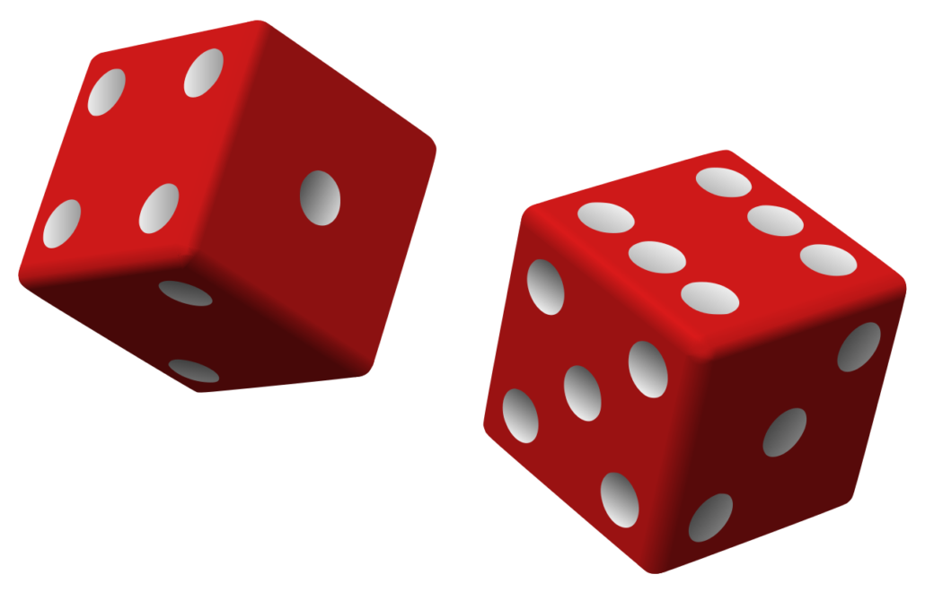
echo $(( (RANDOM % RANGE) + START ))For example, to simulate 10 rolls of a 6 sided dice:
START=1
END=6
RANGE=$(( END - START + 1 ))
RANDOM=314
for i in $(seq 10); do
   echo -n $(( (RANDOM % RANGE) + START )) " "
done
## 5 4 6 3 2 1 1 2 2 4Checking Sequences from RANDOM
The following code will generate a random sample using bash RANDOM. The sample will be scaled to 1. The generated sample will then be tested using Bartels Rank test, where the null hypothesis is that the sequence is random.
Prepare the test data:
RANDOM=314
# bc interferes with RANDOM
temprandom=$(mktemp temp.random.XXXXXX)
for i in $(seq 1000); do
   echo "scale=2;$RANDOM/32768"
done > $temprandom

cat $temprandom | bc | awk '{printf "%0.2f\n", $0}' > bash.random

rm $temprandom
bashText <- readLines(con <- file(paste0(getwd(), '/bash.random')))
close(con)
bashRandom <- as.numeric(bashText)Show first 10 values:
head(bashRandom, n = 10)## [1] 0.05 0.59 0.02 0.84 0.17 0.69 0.41 0.51 0.94 0.55Plot the sequence versus value from RNG:
bashDF <- data.frame(sequence = seq(length(bashRandom)), RANDOM = bashRandom)
ggplot(bashDF, aes(x = sequence, y = RANDOM)) +
   geom_point(size = 0.5, colour = I('purple')) +
   ggtitle('bash RANDOM') +
   theme(plot.title = element_text(hjust = 0.5))
Run Bartels Rank test:
bartels.rank.test(bashRandom, 'two.sided', pvalue = 'beta')##
## Bartels Ratio Test
##
## data: bashRandom
## statistic = -1.116, n = 1000, p-value = 0.2646
## alternative hypothesis: nonrandomnessResult
With a p-value > 0.05 there is weak evidence against the null hypothesis of randomness.
awk rand()
The following code will generate a random sample using the rand function from GNU Awk. This function generates random numbers between 0 and 1. . The generated sample will then be tested using Bartels Rank test, where the null hypothsis is that the sequence is random.
Example (as before rand() is seeded).
echo | awk -e 'BEGIN {srand(314)} {print rand();}'## 0.669965If you don’t specify a seed in srand() it will not return the same results.
You can also generate random integers in a range. For example, to simulate 10 rolls of a 6 sided dice:
echo | awk 'BEGIN {srand(314)} {for (i=0; i<10; i++) printf("%d ", int(rand() * 6 + 1));}'## 5 2 2 5 3 6 1 6 5 5Checking Sequences from awk rand()
Prepare the test data:
seq 1000 | awk -e 'BEGIN {srand(314)} {printf("%0.2f\n",rand());}' > awk.random

awkText <- readLines(con <- file(paste0(getwd(), '/awk.random')))

close(con)

awkRandom <- as.numeric(awkText)
Show first 10 values:
head(awkRandom, n = 10)## [1] 0.67 0.33 0.22 0.78 0.40 0.84 0.11 0.94 0.70 0.68Plot the sequence vs value from RNG:
awkDF <- data.frame(sequence = seq(length(awkRandom)), rand = awkRandom)

ggplot(awkDF, aes(x = sequence, y = rand)) +
   geom_point(size = 0.5, colour = I('purple')) +
   ggtitle('awk rand()') +
   theme(plot.title = element_text(hjust = 0.5))
Run Bartels Rank test:
bartels.rank.test(awkRandom, 'two.sided', pvalue = 'beta')##
## Bartels Ratio Test
##
## data: awkRandom
## statistic = 0.29451, n = 1000, p-value = 0.7685
## alternative hypothesis: nonrandomnessResult
With a p-value > 0.05 there is weak evidence against the null hypothesis of randomness.
urandom device
The final tool is the /dev/urandom device. The device provides an interface to the linux kernel’s random number generator. This is a useful tool as it can generate a wide variety of data types.
For example, to print a list of unsigned decimal using od(1):
seq 5 | xargs -I -- od -vAn -N4 -tu4 /dev/urandom## 2431351570
## 2713494048
## 2149248736
## 2371965899
## 4265714405It can also be used to source random hexadecimal values:
seq 5 | xargs -I -- od -vAn -N4 -tx4 /dev/urandom## 5dd6daf1
## 819cf41e
## c1c9fddf
## 5ecf12b0
## cae33012Or it can generate a block of 64 random alphanumeric bytes using:
cat /dev/urandom | tr -dc 'a-zA-Z0-9' | fold -w 64 | head -n 5## Rui7CImJglwzzoB4XNKljLPe0WPX7WZLDy1PGl6nxkwcttTNrPDwly3d5tXTQfpp
## VhdEVxX6Il8DOTY4rKISrW5fyqF7AeZmbTwKxwd8Ae2SCEwINiRkeQVtzeXY2N8j
## pZFVpBHEEZawu6OQ52uNzRVaI5qqbDeoXKbR0R8jeGKTRcqPlKEpSFv5UaFJgo5w
## SGN6dh03OJMF8cVDPrOTcDhL1esDpK2FJl2qnIW67A9hKedIPukVHJp0ySBlvTWY
## zLH9thMYXYK6qi6IRF8vw5iXaiWut1ZT9BazJfzyCGYTxPMxmOCHIqUt2yyTrAQDChecking Sequences from urandom
To create a test sample that is scaled to 1, I will sample two digits from urandom and use these as decimal values. The generated sample will then be tested using the Bartels Rank test, where the null hypothesis is that the sequence is random.
Prepare the test data:
cat /dev/urandom | tr -dc '0-9' | fold -w2 | \
    awk '{printf("0.%02d\n",$1)}' | head -1000 > urandom.random
urText <- readLines(con <- file(paste0(getwd(), '/urandom.random')))
close(con)
urRandom <- as.numeric(urText)Show first 10 values:
head(urRandom, n = 10)## [1] 0.78 0.62 0.03 0.03 0.66 0.36 0.75 0.34 0.91 0.81Plot the sequence vs value from RNG:
urandomDF <- data.frame(sequence = seq(length(urRandom)), urandom = urRandom)
ggplot(urandomDF, aes(x = sequence, y = urandom)) +
   geom_point(size = 0.5, colour = I('purple')) +
   ggtitle('/dev/urandom') +
   theme(plot.title = element_text(hjust = 0.5))
Run the Bartels Rank test:
bartels.rank.test(urRandom, 'two.sided', pvalue = 'beta')##
## Bartels Ratio Test
##
## data: urRandom
## statistic = -0.668, n = 1000, p-value = 0.5044
## alternative hypothesis: nonrandomnessResult
With a p-value > 0.05 there is weak evidence against the null hypothesis of randomness.
Some final thoughts
Of the tools explored, urandom is the most versatile, so it has broader application. The downside is that its results are not easily reproducible and issues have been identified by a study by Gutterman, Zvi; Pinkas, Benny; Reinman, Tzachy (2006-03-06) for the Linux kernel version 2.6.10.
Personally, this has been a useful learning exercise. For one, it showed the limitations in generating and testing for (pseudo)random sequences. Indeed, Aaron Roth, has suggested:
As others have mentioned, a fixed sequence is a deterministic object, but you can still meaningfully talk about how “random” it is using Kolmogorov Complexity: (Kolmogorov complexity). Intuitively, a Kolmogorov random object is one that cannot be compressed. Sequences that are drawn from truly random sources are Kolmogorov random with extremely high probability.
Unfortunately, it is not possible to compute the Kolmogorov complexity of sequences in general (it is an undecidable property of strings). However, you can still estimate it simply by trying to compress the sequence. Run it through a Zip compression engine, or anything else. If the algorithm succeeds in achieving significant compression, then this certifies that the sequence is -not- Kolmogorov random, and hence very likely was not drawn from a random source. If the compression fails, of course, it doesn’t prove that the sequence has high Kolmogorov complexity (since you are just using a heuristic algorithm, not the optimal (undecidable) compression). But at least you can certify the answer in one direction.
In light of this knowledge, lets run the compression tests for the sequences above:
ls -l *.random## -rw-r--r-- 1 frank frank 5000 2019-02-12 09:51 awk.random
## -rw-r--r-- 1 frank frank 5000 2019-02-12 09:51 bash.random
## -rw-r--r-- 1 frank frank 5000 2019-02-12 09:51 urandom.randomCompress using zip:
for z in *.random; do zip ${z%%.random} $z; done## adding: awk.random (deflated 71%)
## adding: bash.random (deflated 72%)
## adding: urandom.random (deflated 72%)Compare this to non-random (trend) data:
for i in $(seq 1000); do printf "0.%02d\n" $(( i % 100 )) ; done< > test.trend
zip trend test.trend
## adding: test.trend (deflated 96%)Or just constant data:
for i in $(seq 1000); do echo 0.00 ; done > test.constant
zip constant test.constant
## adding: test.constant (deflated 99%)So zipping is a good, if rough, proxy for a measure of randomness.
Stay tuned for part two to discover how random data can be used in testing code.
